Data Downloading, Interoperability, and Working with Projections in Python

Lab #5: Data Downloading and Management

Introduction:

The goal of this activity is to become familiar with the process of gathering data in different formats from different providers online and using them in ArcMap. To do this one has to be able to join and project that data into the same coordinate system as well as designing and building a geodatabase to hold that data. The downloaded and managed data is then to be turned into displays illustrating different aspects of Trempealeau County topology.

Methods:

1.   1)Download the data.

a.       Data was gathered from the following sources to conduct maps of Trempealeau County.

b.      US Department of Transportation-Bureau of Transportation Statistics-Railway Network

                                                               i.      http://www.rita.dot.gov/bts/sites/rita.dot.gov.bts/files/publications/national_transportation_atlas_database/index.html

c.       USGS National Map Viewer-National Land Cover

                                                               i.      http://nationalmap.gov/about.html

d.      Trempealeau County Land Records-Land Use

                                                               i.      http://www.tremplocounty.com/tchome/landrecords/

e.      USDA NRCS Web Soil Survey-Soils Data

                                                               i.      http://websoilsurvey.sc.egov.usda.gov/App/HomePage.htm

f.        USGS-Elevation in High resolution

                                                               i.      http://www.mrlc.gov/

g.       Accuracy of this data in a comparison table is below as figure 1.

Figure 1: An Excel table comparing accuracy to data sources used in this activity.

2)These different DEMs. TIFs, and mosaic files had to be put into a constructed geodatabase so that they could be managed easiest. Several tools and several attempts were gone through in order to arrive at the goal of having all rasters combined in one area in the geodatabase. The rasters also all had to be in “.tif” format to enable combinations and loops to be run on them in Python. Once in “.tif” format they were placed in the same location in the geodatabase. Entitled “images”, the .tif folder enabled a Python script to locate and manipulate the images.

3) The data is then imported and joined based on common attributes so that it can be displayed. This is done using a Python script, the script is figure 2.

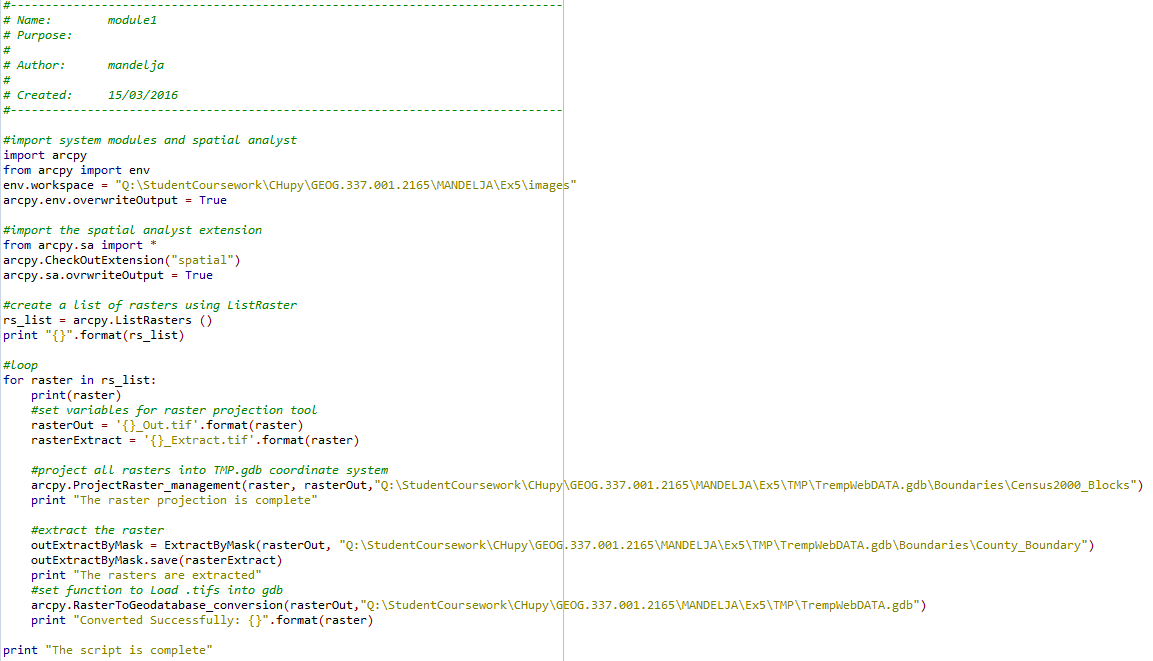
Figure 2: The Python script for combining and extracting the rasters. 

4)The output of the script run created the images needed to display crop type, land use, and elevation. A map of each is below as figures 4-6 with a locator map of Trempealeau County Wisconsin as figure 3.

Figure 3: Trempealeau County in Wisconsin-the area of interest.

Figure 4: An elevation map by meters of the county.

Figure 5: Land Cover in Trempealeau County.

Figure 6: Crop type from the USDA dataset.

Discussion and Conclusion:

The resulting maps display the wealth of knowledge and information that can be gathered from just one county in Wisconsin. This project displays the use of online resources to create products that can be used for multiple different analysis of the land. This particular group of data will go towards analyzing frac sand mines across the county but there are more applications and the method of collecting and organizing the data was a great step farther into online data management. There were some errors as far as data accuracy goes, the metadata was not always consistent or accurately recorded which could leave holes in an argument propped up by the data. The biggest issue with this lab happened when running the python script. There were several attempts to complete the script and correct the multiple errors. Errors occurred in file naming, a selected file started with a number which cannot happen. File location was also an issue as files must all be in the same folder in the same geodatabase and in the same format in order to run the “loop” that was needed. Eventually the issues were resolved but this was certainly the most difficult segment of the lab.