Raster Suitability

Building a Suitability Raster for Mine Placement

Introduction: 

The goal of this activity is to create multiple raster outputs for Trempealeau County (figure 1) in regards to frac mine location. The county is in the southwest region of Wisconsin and has the southern tip of the county touching the Mississippi River. Due to the geoprocessing ability of the computers being used and the time required, only the southern half of the county will be analysed though the same processes could be run on the northern portion as well. Models will be created to show where mining is desirable and where mining is more dangerous. A final map should be able to display the best location for mines with the least impact on humans and the environment.

Figure 1: The area of interest is Trempealeau County Wisconsin.

Objectives:

Suitability of mining:

1. geologic criteria
2. land use/cover criteria
3. distance to railroads 
4. appropriate slope
5. water table depth 
6. Combine 1-5 into a display

Dangerous Mining:

1. Impact on streams
2. impact on ideal farmland
3. impact on residential and populated areas
4. impact on schools
5. impact on wildlife areas
6. Combine 1-5 into a display

Methods:

The process for this lab is to use model builder to create a workflow to take several different feature classes and arrive at the result of a suitability model. To do this the required features to determine quality of mining were added to model builder and reclassified. The reclassify tool allows the map maker to break down the feature class from the original values to simply desirable or undesirable, this allows for simpler input in the raster calculator and makes the suitability level in each layer more visible. The workflow, figure 2, is for the suitability raster for mine placement. Since this did not work and resulted in the crashing of ArcMap continuously the maps created to go into the raster calculator are included in figure 3.

Figure 2: The set up for the model builder for suitability.

Figure 3: These maps combine to show the ideal placement for frac mines.

After suitability was calculated the next step was to figure out where mines could not be located, these were areas that would impact schools, residential areas, wildlife areas, streams, and farmland. The same workflow idea was used with this impact calculator except this time it was to figure out where would not work as opposed to where would work. This model ran smoother and allowed me to run raster calculator. The workflow, figure 4, shows the steps run in model builder though several steps were done outside the model to prepare it for the model. The final output, figure 5, is where the mines could not go, the risk index on the final map display areas to avoid when mining. 

Figure 4: This workflow was used in model builder to calculate mining risk.

Figure 5: The final impact maps.

Conclusion:

When all of the tools were done running the result is a collection of maps that shows where a mine should be placed and another collection pointing to where mines should not be placed. Had the first raster calculator worked it would have shown, as it does in figure 5, a final map with a summary of the maps showing where to place a mine. 

Discussion:

This was one of the most frustrating projects I have yet done. There were continuous shutdowns and crashes by ArcMap and several of the tools, mainly euclidean distance and raster calculator persisted to not run. In the end the result for the impact on mining was as desired. This lab, even in its non-perfection, required an immense amount of work and trouble shooting.  

The sources for the information used in the maps are sited on the maps themselves.

Frac Mines and Network Analysis

Network Analyst with Frac Sand Mines

Introduction:

The goal of this exercise is to run network analysis of the roads used to connect frac mines to rail terminals. Routing using the analyst will be done to determine which roads are used by how many mines, this will allow a damage estimate for the roads to be given as well as a cost for maintenance. To measure the impact and cost on the county roads the following workflow was used:

1) Determine what terminal the sand from each mine will go to to be put on a rail car

2) Determine the most efficient route to each terminal

3) Calculate the length of the route by county

4) Estimate the costs for each county for road maintenance 

Additional background for how this process would be run was gathered from reading sections of "Transportation Impacts of Frac Sand Mining in the MAFC Region: Chippewa County Case Study" published by the National Center for Freight and Infrastructure Research and Education. 

Methods:

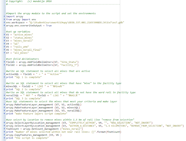
The first step in this project was running a python script to prepare the multiple layers of data to go into network analyst. The script ran on all of the mines in the data set to come up with the mines that were desired. These mines had to fit the criteria of being an active mine, not having a rail loading station, and they had to be farther than 1.5 km from a rail line. The script had to be written to account for the multitude of variables within the geodatabase, a screenshot of the script is below as figure 1.

Figure 1: This python script was run to determine which mines throughout the whole state fit the desired criteria.

The next step in the project was to determine which of the mines, found using the python script, would be routed to which rail terminal for distribution and processing. Instead of running a long list of tools within arcmap, model builder was utilized to use network analyst to find the shortest routes for the trucks. Once that was found calculations were done within the fields of data to determine the mileage each road would see as a result of routing and a simple formula of 2.2 cents per mile was used to calculate road repair and maintenance cost from the high use by sand trucks. The workflow in model builder is figure 2 showing how many steps, additions, and tools this process required.

Figure 2: The workflow created in model builder to answer the research question.

Results:

The "Closest Facility" function run in the model builder created the information output to go into the display of figure 3, a map of the best routes for each facility to send its trucks on to get to a terminal. 

Figure 3: This map displays the best routes for frac sand trucks to take to rail terminals.

The next step was to determine the cost of each truck route in each county. This would show how much money it is going to cost the county to have upkeep on the road each year. This was done by using the "length" field to calculate from meters to miles then, assuming each truck does 100 trips a year, multiplying the miles by 100. That final miles measurement is then multiplied by $.22 for each mile the truck travels. The resulting table of figures can be seen in figure 4 and the map of those figures displaying the cost is in figure 5.

Figure 4: This is a screenshot of the attribute table of the calculations done in model builder.

Figure 5: This map displays, by counties relevant to the study, how much road maintenance will cost in US dollars.

Conclusion/Discussion:

The final answer is displayed by figure 6, a graph of the costs per county, and is displayed by figure 5. The cost of running and routing frac sand in trucks on county roads ads a considerable cost to a budget that must be accounted for. Of course this cost analysis doesn't account for environmental long term cost but it does give an idea on some level of the impact on roads. If this project were done again it would be interesting to see how much the counties budgeted for road repair and how much of that budget was going to repair frac mine frequented roads. This could also be calculated in model builder. 

Figure 6: This graph compares each county's cost to the other county's cost for road maintenance on the routes within the county.

This project used a combination of python and model builder to create outputs to answer a spatial question. Though initially difficult to work with the python and model builder offers an efficient and visible way to work the data instead of running it all by tools. This was a great way to get more acquainted with each form of software to run arcmap and I am certainly more comfortable with it at this point. It was helpful to see how such a complex question could be answered without running endless tools by hand. The focus, network analyst, seemed to me to very similar to how google maps routes and in many ways it is. This is such a complex service that understanding how it works on this level is fascinating and offers a lot of insight into how GIS and network analyst specifically can be practically applied to so many of today's issues. 

Sources:

Hart, Maria, Teresa Adams, and Adrew Schwartz. "Transportation Impacts of Frac Sand Mining Ie MAC Region: Chippewa County Case Study." National Center for Freight & Infrastructure Research & Education (2013). Web. 16 Apr. 2016. 

Data Downloading, Interoperability, and Working with Projections in Python

Lab #5: Data Downloading and Management

Introduction:

The goal of this activity is to become familiar with the process of gathering data in different formats from different providers online and using them in ArcMap. To do this one has to be able to join and project that data into the same coordinate system as well as designing and building a geodatabase to hold that data. The downloaded and managed data is then to be turned into displays illustrating different aspects of Trempealeau County topology.

Methods:

1.   1)Download the data.

a.       Data was gathered from the following sources to conduct maps of Trempealeau County.

b.      US Department of Transportation-Bureau of Transportation Statistics-Railway Network

                                                               i.      http://www.rita.dot.gov/bts/sites/rita.dot.gov.bts/files/publications/national_transportation_atlas_database/index.html

c.       USGS National Map Viewer-National Land Cover

                                                               i.      http://nationalmap.gov/about.html

d.      Trempealeau County Land Records-Land Use

                                                               i.      http://www.tremplocounty.com/tchome/landrecords/

e.      USDA NRCS Web Soil Survey-Soils Data

                                                               i.      http://websoilsurvey.sc.egov.usda.gov/App/HomePage.htm

f.        USGS-Elevation in High resolution

                                                               i.      http://www.mrlc.gov/

g.       Accuracy of this data in a comparison table is below as figure 1.

Figure 1: An Excel table comparing accuracy to data sources used in this activity.

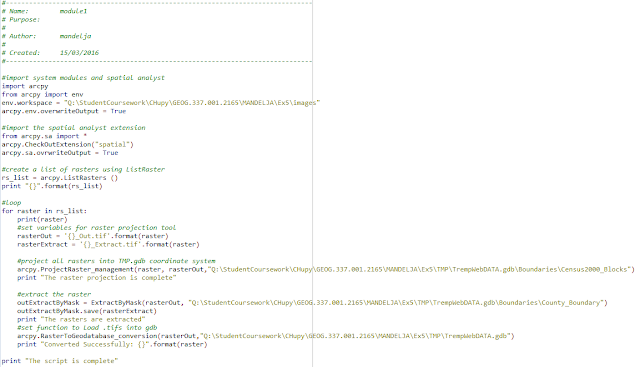
2)These different DEMs. TIFs, and mosaic files had to be put into a constructed geodatabase so that they could be managed easiest. Several tools and several attempts were gone through in order to arrive at the goal of having all rasters combined in one area in the geodatabase. The rasters also all had to be in “.tif” format to enable combinations and loops to be run on them in Python. Once in “.tif” format they were placed in the same location in the geodatabase. Entitled “images”, the .tif folder enabled a Python script to locate and manipulate the images.

3) The data is then imported and joined based on common attributes so that it can be displayed. This is done using a Python script, the script is figure 2.

Figure 2: The Python script for combining and extracting the rasters. 

4)The output of the script run created the images needed to display crop type, land use, and elevation. A map of each is below as figures 4-6 with a locator map of Trempealeau County Wisconsin as figure 3.

Figure 3: Trempealeau County in Wisconsin-the area of interest.

Figure 4: An elevation map by meters of the county.

Figure 5: Land Cover in Trempealeau County.

Figure 6: Crop type from the USDA dataset.

Discussion and Conclusion:

The resulting maps display the wealth of knowledge and information that can be gathered from just one county in Wisconsin. This project displays the use of online resources to create products that can be used for multiple different analysis of the land. This particular group of data will go towards analyzing frac sand mines across the county but there are more applications and the method of collecting and organizing the data was a great step farther into online data management. There were some errors as far as data accuracy goes, the metadata was not always consistent or accurately recorded which could leave holes in an argument propped up by the data. The biggest issue with this lab happened when running the python script. There were several attempts to complete the script and correct the multiple errors. Errors occurred in file naming, a selected file started with a number which cannot happen. File location was also an issue as files must all be in the same folder in the same geodatabase and in the same format in order to run the “loop” that was needed. Eventually the issues were resolved but this was certainly the most difficult segment of the lab. 

Geocoding of Frac Mines

Lab #6: Geocoding Frac Sand Mines in Wisconsin

Introduction:

The purpose of this lab activity is to utilize the geocoding toolset to place active and inactive frac sand mines across the state of Wisconsin and compare the geocoded dataset to the actual locations of the mines. Each student was given a grouping of roughly 16 random mines with the purpose of using the broken information given, and creating a more accurate dataset with geocoding. The original Excel file can be seen below in figure 1, clearly not all mines have a complete usable address. The geocoded addresses will then be compared to the real accurate locations of the mines to see how accurate the geocoding was.

Figure 1: The provided Excel file before normalization.

Methods:

In order to geocode the original data and analyse accuracy several steps had to be done. The first step is to normalize the data.

1) Data normalization was done with the mine addresses so that the needed information was more easily accessed and the mines could be found with what information was given. A normalized table can be seen in figure 2. When comparing the original and normalized file it is clear how sporadic and inconsistent the provided data is.

Figure 2: A screenshot of the normalized data. The amount of fields containing "n/a" show how inconsistent the provided data was.

2) Geocoding begins with the step of accessing the geocoding toolbar. From the toolbar “geocoding addresses” is selected and the normalized sheet is added into the address field. “Address Inspector” is used to see which addresses in the table match to locations, my personal file for geocoding had 12 matched addresses and 4 unmatched. The unmatched addresses were found with the public land survey system, or PLSS, and “Pick Address from Map” was used to match a point to the address.

3) Merging shapefiles is the next step. The members of the class who geocoded the same mine locations as were contained in my file were combined into one shapefile to be compared to the mines I personally geocoded. This way the accuracy of geocoding among peers could be tested.

4) Distancing measuring is possible with several tools. The one used in this case was the “Generate near distance table”. This tool took the location of geocoded points and measured, in meters, the distance to a point that was supposed to be at the same point. The tool creates an output of a table containing the mine information and the distance between the points that is calculated. The result from this tool for the individually geocoded points and peer geocoded points is visible in figure 3. The same process is done for the real and accurate mine locations, a screenshot of the output is below as PLACE FIGURE. 

Figure 3: This table displays, in meters in the "near_dist" attribute, how far away from each other the mines were that were geocoded by me and by my peers.

Figure 4: This table displays, in meters in the "near_dist" attribute, how far away from each other the mines that are placed, by the DNR, at the correct locations.

5) Map. The final step was to take the geocoded files and compare accuracy visually in a map format. The first map, figure 5, is of the points I geocoded compared to others in the class who geocoded the same mines. The second map, figure 6, displays the mines I geocoded in relation to the actual position of those mines.

Figure 5: This map displays the mines that were geocoded by me personally and those done by classmates. Some mines are placed in the same location while others are clearly placed in wrong areas.

Figure 6: This map shows where the mines that were geocoded by me actually are. Again, this shows that some mines were placed by me in the right location while others clearly weren't. 

Discussion:

Of course this method of geocoding is not without its flaws. There are inherent and operational errors that often occur with geographical data in general. The errors came from issues in the data automation and compilation areas including geocoding which was done in this lab. The issue with geocoding is that the points will never be exact because they are manually placed and so they will never be in the exact location as where they actually area. Another error is attribute data entry. This error would not be visible through geocoding but is as simple as being provided with the wrong data in the provided Excel file.

Attribute accuracy, or closeness, is necessary to be able to see which points have been placed in the "right" area. The only way to truly know where exactly a location is is to rely on the longitude and latitude of the point. Only that coordinate can be referenced to to compare a geocoded points closeness.

Conclusion:

When the activity was finished the Excel file had been normalized, the points had been geocoded, mines with only PLSS addresses had been geocoded, and the accuracy of those points was tested using tools in ArcMap. This will be a good exercise to be able to refer to later in work as I will likely need to geocode points and they will not always be perfect. The near distance table tool allows me to see how close the points are to being accurate which is very valuable.

Sources:

Wisconsin Department of Natural Resources. (n.d.). Retrieved November 8, 2015, from http://dnr.wi.gov

PLSS - Legal Descriptions | PLSS. (n.d.). Retrieved November 8, 2015, from http://www.sco.wisc.edu/plss/legal-descriptions.html 

       

Python

Python Demonstrations

Python Demo:

The purpose of this first demonstration was to learn about the purpose of using python in relation to running functions in ArcMap and how to connect python to the geoprocessing environment. This demo was done entirely within ArcMap using the Python scripting window. This window allows for small amounts of code to be run directly in ArcMap for ease of use. Three actions were done using this method including two buffers and a clip to a provided geodatabase of "random" points in Michigan. One the three process had been run successfully the demo was complete. 

Since this particular demo was done in ArcMap and a text file was not saved a screenshot is provided below to show the recall of the projects run as they appeared as a Python script. 

Python Demo 2:

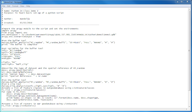
The second demonstration for Python scripting saw the introduction of PyScripter and ArcPy. Instead of needing to write the code within ArcMap, PyScripter enables the writer to write longer codes and check them as codes are written then the final code can be run and applied to ArcMap. This demo included the skills of editing a script template, setting up a script, and printing a statement. 

Below is a copied HTML text of the created script made in PyScripter and applied in ArcMap.

Python Demo 3:

In the third python demo more advanced PyScripter was practiced. Setting variables and running a tool to describe the data was put into application. This step delved deeper into how many different things PyScripter can actually do and how it can apply to spatial questions.

This is a text file of the run python code created in PyScripter:

Python for Mines in Ex 7:

This python script was constructed to run within a geodatabase with rail terminals, mines of any status, and rail lines. The goal was to use a script to find how many mines were not within 1.5 km of a rail line and still within Wisconsin. The number of mines that fit this criteria was found. The script ran and using a statement a print of how many features would be selected was had and the resulting layer contained 47 mines. Below is the script in a screenshot format.

Frac Sand Mining

Frac Sanding in Wisconsin

By: Joseph Mandelko

 

            For over 60 years a method of oil and natural gas extraction has been used called hydraulic fracturing, or fracking. The process uses a mixture of pure quartz sand and water under extreme amounts of pressure to open fissures far below the surface of the earth allowing for natural gas and oil to be accessed easier than before. Recently there has been a development in the discipline of fracking that has resulted in even more resources being able to be extracted. This advancement is the idea of horizontal drilling. Now, with just one well drilling, the extraction company can send out frack lines horizontally from the initial drill point allowing for resources in the vicinity of the drill point to be accessed.

            In the state of Wisconsin, as with many other states with similar geologic formations, the increase in popularity of frac sanding has begun to be noticeable. Figure 1 below shows the location of frac sand mines and processing plants in Wisconsin as of 2013. The most important segment of the map however is the sandstone formations shown, this is a huge indicator of the future of fracking in the state. The western side of the state shows a huge potential to be mined not just for oil and natural gas but more importantly for the pure quartz sand needed in frac mining. The geologic feature of such a stable and constant sandstone layer has drawn attention by mining companies and the effects are all across the board.

            Because of the proximity and ease of use of the railroad systems in Wisconsin the state has easier accessibility and transportation of mined sand than even neighboring Minnesota. On one hand this has been good for Wisconsin by creating jobs and pumping money into the state’s economy. On the other hand the heavy use of mining equipment has begun to have effects on the environment and populations near mining operations. The proximity of the mines to communities has resulted in increased lung cancer, and other illness associated with dirty air. There is also the fact that trucks, in many cases run constantly all day and night in and out of mines to remove the sand mined from the mine. This has caused overall quality of life to decline dramatically and communities are facing hard decisions on allowing or banning frac mining in their townships.

            Geographic information systems can be, and are, used heavily in the area of mining and it is no different for frac mining. Data from the USGS and local county level data can be combined to display anything from current mining areas and effected communities. The issue of sand transportation can also be displayed to show where heavily traveled roads are and what the effect of the traffic is on local communities. GIS can also be used to discover where better, less intrusive, routes are located to help reduce issues with health and the community. In this class we will use GIS to analyses the department of transportation data on Trempealeau County to look at the impacts of mining on the roads and communities there.   

 

 

(Figure 1: Location of sandstone formations and frac sand mines and processing plants. Wisconsin Geologic and Natural History Survey)

 

Sources:

Hart, Maria, Teresa Adams, and Andrew Schwartz. "Transportation Impacts C Sand Mining in the MAFC Region." National Center for Freight & Infrastructure Research & Education (2013): n. pag. Web. 24 Feb. 2016.

Parsen, Mike, and Jay Zambito. "Mining: Frac Sand." Wisconsin Geological Natural History Survey. Wisconsin Department of Natural Resources, n.d. Web. 27 Feb. 2016.

Younger, By Sally. "Sand Rush: Fracking Boom Spurs Rush on Wisconsin Silica." <i>National Geographic</i>. National Geographic Society, n.d. Web. 27 Feb. 2016.